ホイン法

ホイン法（Heun’s method） または 改良オイラー法（Improved Euler’s method） はオイラー法で利用する始点 \(t\) での関数の傾きの代わりに，始点 \(t\) と終点 \(t+h\) での傾きの平均を用いて近似を行う．つまり，

\[ \begin{aligned} x(t+h) = x(t) + \frac{h}{2} \left \{ f\left (x \left (t \right),t\right)+ f\left (x + hf\left(x,t\right),t + h\right)\right \} \end{aligned} \]

の近似式を利用する．

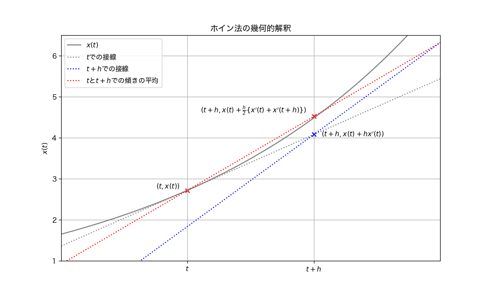
オイラー法と同様にこの近似式の幾何的解釈を図に示す．ホイン法では始点 \(t\) での傾き（図の灰色の点線）に加えて，終点 \(t+h\) での傾き（図の青色の点線）の情報を利用する．近似式からもわかるように，これらの傾きを平均した傾きを使って次の時刻 \(t+h\) での関数の値を外挿する（図の赤色の点線）．これを数値列の近似として書くと，

\[\begin{split} \begin{aligned} \tilde{x}_{i+1} &= x_i + hf\left(x_i,t_i \right) \\ x_{i+1} &= x_i + \frac{h}{2} \left \{ f\left(x_i,t_i \right) + f\left(\tilde{x}_{i+1},t_{i+1} \right)\right \} \end{aligned} \end{split}\]

となる．ホイン法は二次の精度をもつ近似法として知られている．このことは次のようにオイラー法から修正した導関数，つまり，次の時刻の関数の値 \(f(x+hf(x,t),t+h)\) のTaylor展開をすることで確認できる．二変数関数であることに注意すると

\[ \begin{aligned} f(x+hf(x,t), t+h) = f(x,t)+h \frac{\partial f}{\partial t} + h\frac{\partial f}{\partial x} \frac{dx}{dt} +O(h^2) \end{aligned} \]

となる．続いて，これをホイン法で用いた近似式に代入する．

\[\begin{split} \begin{aligned} x(t+h) &= x(t) + \frac{h}{2} \left \{ f\left (x \left (t \right),t\right)+ f\left (x\left(t\right) + hf\left(x,t\right),t + h\right)\right \} \\ &= x(t) + \frac{h}{2} \left \{ f\left (x \left (t \right),t\right)+ f(x(t),t)+h \frac{\partial f}{\partial t} + h\frac{\partial f}{\partial x} \frac{dx}{dt}+O(h^2)\right \} \\ &= x(t) + h f\left (x \left (t \right),t\right) + \frac{h^2}{2} \left \{ \frac{\partial f}{\partial t} + \frac{\partial f}{\partial x} \frac{dx}{dt} \right \} + O(h^3) \\ &= x(t) + h x'(t) + \frac{h^2}{2} x''(t) + O(h^3) \end{aligned} \end{split}\]

ここで \(f(x(t),t)=x'(t)\) であり，\(x(t)\) の二階導関数が

\[ \begin{aligned} x''(t)=\frac{d^2 x}{d t^2}=\frac{\partial f}{\partial t}+\frac{\partial f}{\partial x} \frac{d x}{d t} \end{aligned} \]

であることを利用した．式からもわかるように右辺第3項まで \(x(t+h)\) のTaylor展開と一致しており，ホイン法が二階の導関数までを含む二次近似をしており，オイラー法より優れたアルゴリズムであることがわかる．

ホイン法の実装

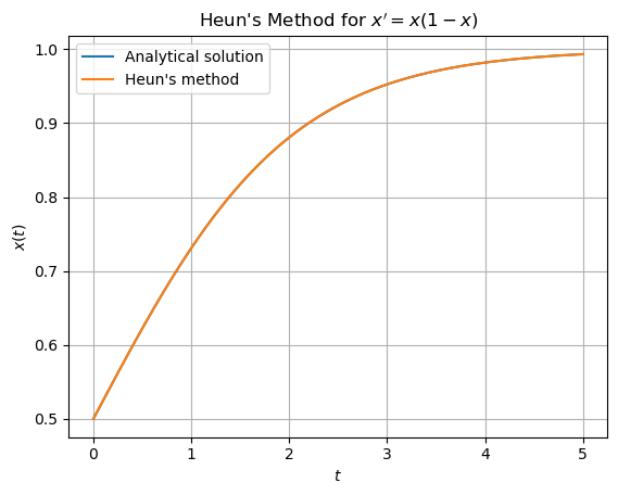
これをPythonで実装する．今回は次の初期値問題を解く

\[ x'=x(1-x), x(0)=\frac{1}{2} \]

解答：解析解は \(x=\frac{1}{1+e^{-t}}\) であり，以下のプログラムで解析解と近似解の違いをプロットする．

import numpy as np
import matplotlib.pyplot as plt

def heun_method(f, x0, t0, tn, h):
    """
    ホイン法（修正オイラー法）を用いて常微分方程式を数値的に解く関数
    :param f: 常微分方程式の右辺の関数 f(t, x) 
    :param x0: 初期値 x(t0)
    :param t0: 初期時刻
    :param tn: 最終時刻
    :param h: 刻み幅
    :return: 時刻と近似解のリスト
    """
    t_values = [t0] # t_0の値を格納したリストを作成
    x_values = [x0] # x_0の値（初期値）を格納したリストを作成
    
    t = t0
    x = x0
    
    while t < tn: # 最終時刻になるまで繰り返す
        # 時刻と式()に基づく値の更新
        k1 = h * f(t, x)
        k2 = h * f(t + h, x + k1)
        x = x + 0.5 * (k1 + k2)
        t = t + h
        
        # 計算された値をリストに追加
        t_values.append(t)
        x_values.append(x)
        
    return t_values, x_values

# 微分方程式の右辺
def f(t, x):
    return x * (1 - x)

# 解析解
def analytical_solution(t):
    return 1. / (1 + np.exp(-t))

# 初期値とパラメータ
x0 = 0.5 # 初期値
t0 = 0 # 開始時刻
tn = 5 # 終了時刻
h = 0.001 # 刻み幅

plt.figure()
t_analytical = np.linspace(t0, tn, 500) # 区間[開始時刻,終了時刻]で時刻を500点サンプリング
x_analytical = analytical_solution(t_analytical) # 解析解の計算
plt.plot(t_analytical, x_analytical, label='Analytical solution') # 解析解のプロット 

t_values, x_values = heun_method(f, x0, t0, tn, h) # ホイン法の計算
plt.plot(t_values, x_values, label="Heun's method") # ホイン法の結果のプロット
plt.title(r"Heun's Method for $x' = x(1-x)$")
plt.xlabel(r'$t$')
plt.ylabel(r'$x(t)$')
plt.grid(True)
plt.legend()
plt.show()

Intel MKL WARNING: Support of Intel(R) Streaming SIMD Extensions 4.2 (Intel(R) SSE4.2) enabled only processors has been deprecated. Intel oneAPI Math Kernel Library 2025.0 will require Intel(R) Advanced Vector Extensions (Intel(R) AVX) instructions.
Intel MKL WARNING: Support of Intel(R) Streaming SIMD Extensions 4.2 (Intel(R) SSE4.2) enabled only processors has been deprecated. Intel oneAPI Math Kernel Library 2025.0 will require Intel(R) Advanced Vector Extensions (Intel(R) AVX) instructions.